Over the last twenty years or so, latent class modeling has replaced hierarchical cluster modeling as the go-to methodology for market segmentation studies. The reasons for this are many: the ability to include variables of differing scales, the availability of clear statistical criteria with which to evaluate segment quality and quantity and, most of all, clarity and actionability of the resulting segments. While the benefits are clear, the conceptual underpinnings of the methodology are not so obvious to non-specialist audiences. This makes it difficult to communicate aspects that are unique to latent cluster models, particularly the distinction between Indicators (or endogenous variables) and Covariates (or exogenous variables), which are absent in traditional clustering methods. The goal of this article is to provide an intuitive description of the methodology, along with examples using simulated data to illustrate the relevant concepts.
Proximity versus Probability
It is helpful to begin our discussion by understanding the key distinction between traditional hierarchical clustering methods and latent cluster models. The former is based on grouping people together based on how “close” they are to one another using Euclidean measures of distance. A common clustering approach, agglomerative hierarchical clustering[1] starts by assuming every respondent belongs to a separate cluster and then groups people who are close to each other based on a proximity matrix. A proximity matrix is simply an n by n grid of distances between n respondents, where the diagonal is zero, representing the fact that the distance of a point with itself is always zero. The off-diagonal elements are the distance between each respondent on the measured variables. There are various ways to measure this distance (or similarity) and the right measure depends on the shape of the clusters and is not always obvious. The algorithm works by grouping together people with the smallest distance amongst them into a single cluster and then recreating a new proximity matrix. This process continues until the algorithm reaches a pre-specified number of clusters.
In contrast, the underlying principle of latent class modeling is that the data contains a mixture of several distributions and the goal of analysis is to “un-mix” the distributions and assign people to the distribution from which they were most likely to have been drawn. That is, in place of somewhat arbitrary measures of distance, we use a probabilistic framework to assign people into latent classes (i.e. unobserved segments) based on the observed data (i.e. the Indicator variables). This idea of uncovering latent variables based on observed variables is quite widespread in multivariate statistics and is the basis of commonly used techniques in market research, such as Factor Analysis and Structural Equation Modeling (SEM). Factor Analysis helps uncover the underlying constructs such as “price conscious” or “brand driven” that are indicated by observed attitudes and SEM goes a step further and uncovers the relationships amongst these unobserved constructs. When it comes to latent-cluster models, the unobserved variable is discrete, with k-classes, with each class representing a segment.
A reasonable probability is the only certainty
This quote from E.W. Howe encapsulates what statistical analysis is fundamentally about. As everyone who has done at least an introductory course in statistics knows, most commonly observed phenomena follow distributional patterns with specific parameters, the most well-known being the normal distribution, whose parameters are the mean and the standard deviation. As discussed in the previous section, the goal of latent cluster modeling is to uncover the probability distributions of specific variables in the data. That is, we believe that the data in our sample are drawn from different distributions, each with its own mean and standard deviation. The trick is to figure out which distribution each data point (i.e. respondent) comes from.
The E-M Algorithm and Bayes Rule
These two concepts are essential in developing an understanding of the mechanics of latent clustering.
In order to simplify the discussion, let us consider a data set containing measurements on a single variable, say respondent height. Further, we believe that the data consists of two distinct groups of people, i.e. the measured heights are drawn from two normal distributions with a unique mean and standard deviation. It is logical to assume that the two distributions correspond to males and females; however, we did not record the gender of the individual. Since we don’t know which distribution any given person is drawn from, we make use of the Expectation Maximization (E-M) algorithm. The E-M algorithm starts by assuming a mean and standard deviation for each of the two distributions. It then looks at each data point individually and computes probabilities that the data point comes from either distribution, given those parameters. The process is elegant in its simplicity: the starting values of the mean and standard deviation can be plugged into the formula for the normal distribution to arrive at P(xi|d1), i.e. probability of data point xi given distribution d1. Bayes Rule is then used to arrive at the posterior probabilities of membership which can then be used to develop updated means and standard deviations and the process starts all over again until convergence is achieved. The prior probabilities, P(d1) and P(d2) can be assumed equal or computed from the data. These posterior probabilities are used to update the starting values of the means and standard deviations and the process starts all over again. We can do this because at the end of step 1, we have a probabilistic assignment of (cluster) membership for each data point. To understand how the starting values are updated, assume that the posterior probabilities were either zero or one. Then the mean of distribution 1 would be the mean of just the data points that have a posterior probability of belonging to distribution 1, and the mean of distribution 2 would be the mean of just those data points that belong to distribution 2. In reality, the updated means are weighted by the probabilities of belonging to each distribution. In this sense, the latent cluster approach is a probabilistic extension of k-means clustering – whereas in K-means, data points are assigned wholly to one centroid or another, here data points have different probabilities of belonging to each distribution.
Bayes Rule
In the previous section, we stated that the E-M algorithm computes probabilities that a given data point comes from one of two distributions. An essential element of this computation utilizes Bayes Rule, named after an 18th century Presbyterian minister and statistician, Thomas Bayes.
In the context of our example, Bayes rule addresses the question, what is the probability of a specific data point, say a height of 61”, coming from distribution 1, i.e. P(d1|61)? Bayes Rule states that:

The corresponding posterior probability that the data point was drawn from distribution d2 is simply P(d2|61) = 1 – P(d1|61).
Note that P(61|d1) and P(61| d2) are computed from the formula for the normal distribution, using the initial estimates for mean and standard deviation we assumed for the two groups. P(d1) is referred to as the prior probability. In the absence of additional information, it is customary to assume equal priors.
Now, it is easier to see how E-M works. Bayes Rule ensures that data points that are “closer” to the d1 distribution will have higher posterior probabilities of belonging to it and vice versa. Therefore, the new mean (and standard deviation) of each distribution will be more influenced by data points that are probabilistically more likely to have come from them respectively. Within reason, it does not matter what the starting values of mean and standard distribution are – the algorithm will “shift” the estimated distributions based on the observed data such that data that are more likely to have come from a particular distribution will contribute more to the parameters of the distribution.
Indicators and Covariates
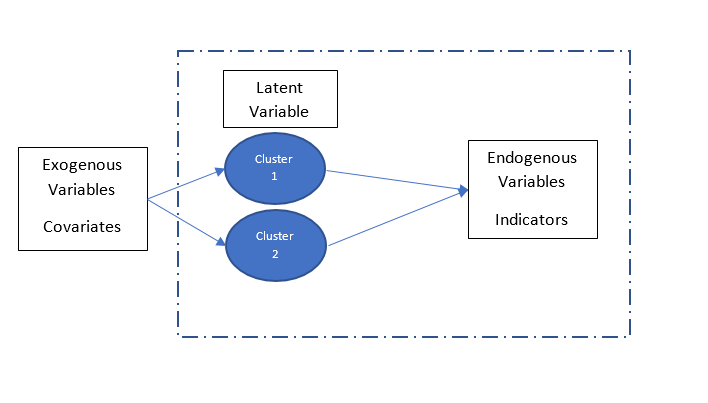
In this example, the height measurement variable is the indicator of the segments. What then is a covariate? The best way to understand the concept of a covariate is as a variable that helps drive class membership. Recall in setting up this example, we stated that we had omitted to record the gender of the individual. However, what if we had recorded estrogen levels? We could enter this into the model for the class membership as a covariate. In other words, covariates help predict the unobserved latent variable which are defined by the distinct distributions of the indicator variables : gender is the unobserved variable, height, the observed Indicator variable is used to derive the male and female distributions and estrogen, the covariate is helpful in predicting which gender a respondent should be assigned to. The schematic below illustrates the relationship across these three variable types:
A simulated data set will help clarify these concepts.
Data Gods with pocket protectors
Simulated data is a great way to gain an understanding of how models work because we can give it specific properties and deprive the model of information that we know in order to evaluate its performance. So, with a wave of our hands (or a line of code) we create a binomial random variable for 1000 cases with a p of 0.5. This will result in a variable with values 0 and 1 that each occur roughly 500 times. We label these male and female respectively. Next, we generate a normally distributed random variable for height, but being data gods, we specify a different mean and standard deviation for males and females. So, in our data, the height variable for males has a mean of 69 inches and a standard deviation of 4.76; the corresponding values for females are 61 and 4.97. We are in essence creating a data set which is a mixture of two distinct normal distributions. Last, we create a normally distributed random variable to capture levels of a hormone called Estradiol with means of 15 for males and 125 for females respectively. We can now test whether the latent cluster model is able to un-mix these two distributions because we know each respondent’s group membership, information that we will withhold from the model.
Model Results
We start by estimating a 2-class latent cluster model using only the simulated height variable as the indicator. This yields one cluster that is 64% of the sample and another cluster that is 36% of the sample. Here are the distributions of males and females (information we withheld from the model) within each cluster:
Chart 1
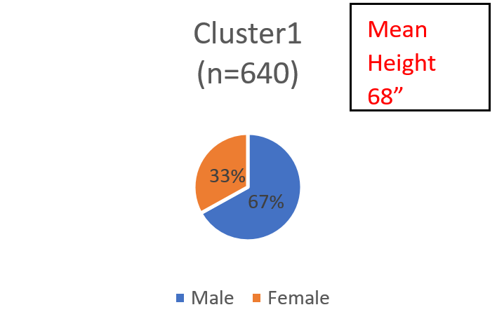

The model has succeeded in identifying a cluster that is predominantly male and another which is predominantly female. It has not, however, completely separated out the males and the females, although the mean heights of each cluster are almost identical to the means in the male and female groups in the simulated data. Upon close inspection, it appears that females who were on the higher end of their distribution end up in cluster 1 and males on the lower end of their distributions end up in cluster 2.
Now, let us estimate another model, with the Estradiol variable entered as an exogenous variable (or co-variate). This model gives us two clusters sized 53% and 47% respectively. Here are the distributions of male and female within the two clusters:
Chart 2
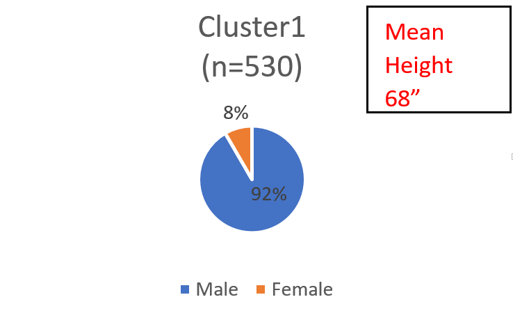
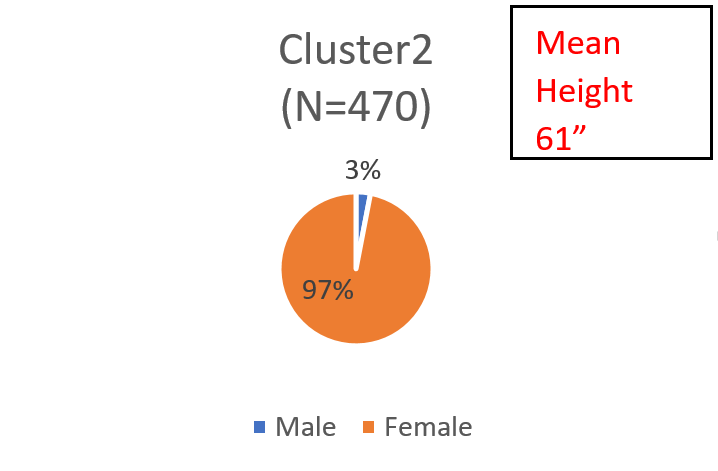
The male-female demarcation is much starker. The addition of the covariate enables the model to more accurately uncover the two distributions that we created, by design. The model has essentially un-mixed the two distributions we had generated! The addition of the covariate enables the model to distinguish the males from the females for those in the overlapping region where they have equal posterior probabilities of coming from either distribution. These results from the simulated data have important implications for the market research analyst:
Segment membership is inherently probabilistic
The parameters of the underlying distributions uncovered by the model are separate from who belongs in each segment. This is because different combinations of data points (or respondents) can yield similar distributional parameters. As we saw in the first model with the simulated data, cluster 1 included females on the high end of their distribution while cluster 2 included males on the low end of theirs. (It helps to visualize two normal curves side by side, the female distribution with the lower mean on the left and the male on the right). Note that from a conceptual point of view, both solutions yield segments with the same underlying characteristics; i.e. taller people in one cluster, shorter in another. Therefore, the question “are these segments real” is irrelevant. If our goal is to market products to people on the taller end of the height spectrum, the first solution will do just as well. We know these clusters are not the “true” clusters we simulated but we do not possess this information in the real world. This leads us to the second point, namely
Covariates do not alter the nature of the segments, merely who occupies them
Covariates impact the probability of cluster membership but do not impact the story underlying each cluster as told by the Indicators. That is, a “cost conscious” segment will remain so regardless of whether it is predominantly male or white or highly educated. The set of covariates we include in the model will simply enable cleaner targeting of the people in the segments, to the extent that there is a measurable relationship between these variables and the latent class membership variable. As we saw in our models using simulated data, the addition of the variable measuring estradiol levels as a covariate helped in predicting class membership more accurately because of its relationship to gender, and gender was the latent variable that yielded the data measured by the Indicator, height. A common misconception is that the indicators variables in the model “determine” the segments. If anything, the opposite is true. That is, it is the latent variable that is responsible for the observed data. Just as an unobservable construct such as an underlying personality type construct results in observable personality traits, the Indicators are manifestations of the underlying process by which the distributions are generated. This is clearly illustrated by our simulated data where we literally created the height variable to be a function of what gender the respondent was.
Indicators, Indicators, Indicators
Data analysis in market research is different from more general “data science” because it is mostly based on a theoretical marketing science/marketing framework. We design surveys to address specific marketing objectives based on what we know of the marketplace such as the market structure, consumer preferences and so on. The attitudinal batteries in a segmentation survey are chosen based on hypotheses regarding consumer behavior, relevant decision drivers and product preferences. For this reason, data analysis is less a fishing expedition than it is an investigation within a carefully constructed framework. Viewed from this perspective, the choice of Indicators is the single most important step in a segmentation (whether latent class or traditional). The most successful segmentation studies I have worked on started with a set of hypotheses and a carefully crafted survey to test them. The team chooses variables based on a similar process of hypothesis generation and an understanding of what it is that the collection of variables represents. Let us revert to our simulated data example. Suppose we had created a normally distributed variable for weight, using the same criterion we did for the height variable. That is, we ensured that men and women have distinct mean and standard deviations. A model which included height and weight along with the estradiol variable would essentially result in the same model as one with just height, i.e. it would uncover the two distributions we had simulated specifically to differ on gender (the simulated data shows this result but it is not reported here). However, what if we created a new variable, BMI, which is based on a specific ratio of height and weight? A latent cluster model based on the BMI variable yields two clusters, sized 69% and 31% respectively with the following gender distributions:
Chart 3
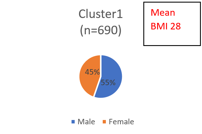
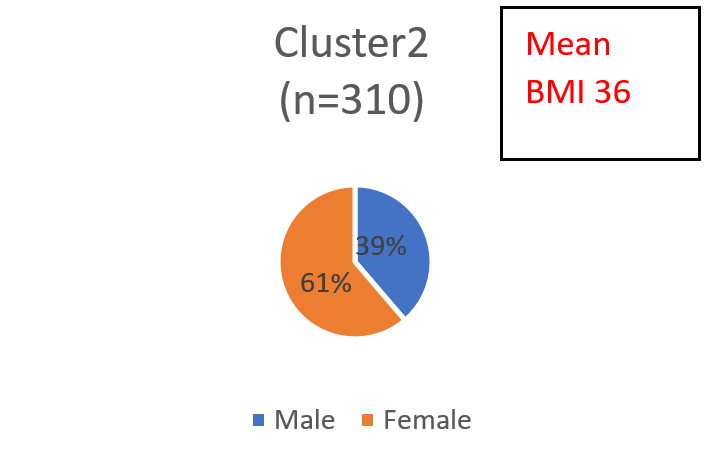
The two clusters (i.e. distributions) uncovered by the model are clearly not distinct on gender, at least not the extent to which the height and weight variables were generated specifically to reflect gender differences. So, which of these segment solutions is the right one? The answer obviously depends on the needs of the marketer – the right solution is the one that is more useful. The key takeaway is that even if certain variables (i.e. height and weight) were the outcome of a specific process (gender), it does not mean that a mathematical combination of those variables is generated by the same process. Segmenting on BMI alone is not the same thing as segmenting on height and weight. This might seem obvious, but it is remarkable how often this is lost in the process of selecting variables for the cluster model. The point is that choosing variables without thought to conceptual underpinnings can have significant impact on the characteristics, and therefore value, of the resulting segments.
Latent cluster modeling is a powerful element of the market research analyst’s tool kit. Its flexibility with regard to scaling of variables and the clarity of resulting segments should make this a first stop for most market segmentation studies. As with all things however, the power and flexibility of the methodology do not obviate the need to follow solid research design principles. Ultimately, the quality of the resulting segments is a function of the thought that goes into survey development and the quality of hypotheses generated by the research team.
[1] Also widely used is K-means clustering in which a pre-specified number of random values are chosen as “centroids” and data points are assigned to each centroid based on a proximity measure. Centroid values are updated based on the data points assigned to each centroid and the process continues until there is no change in the centroids’ position
