
Design Strategies for Pharma Demand Assessment
Introduction
Primary market research is the vehicle of choice (pun unintended) in assessing market potential once a pipeline product gets past the early stages of development. And here, carefully constructed choice/conjoint models rule the roost when it comes to addressing questions of product interest, sensitivity to variations in clinical endpoints and the tradeoffs HCPs make in choosing one treatment versus another and, more crucially, across alternative target product profiles (TPPs).
The specific choice of design, however, is contingent upon various factors. A careful consideration of these factors is critical in ensuring that the demand assessment reflects, as closely as possible, the conditions on the ground that are expected to prevail at launch. To wit, whether the pipeline product:
Is entering an established market, with little to no competitive activity
Is entering a dynamic market with ongoing competitive activity
Is a first entrant in a novel class
Is a later entrant in a new or recently established class
Is in a disease area with a large number of relevant clinical endpoints
Is facing a market with significant access hurdles
The answers to every one of the questions above have a bearing on the choice of research and experimental design. Further, the solution must then weigh task realism and comprehensiveness against the size of the market, feasible sample and associated costs.
The simple case of modeling a single Product X
The simplest case[1] is one where we are testing variations for a pipeline product on eight or fewer clinical end points (attributes) with 2 to 6 levels each. The competitive set is fixed at currently available treatments, and the goal of the choice model is to predict patient share for Product X, given different possible profiles as predicated by the various endpoints being tested. The model itself is straightforward – since the respondent task involves allocation data across Product X and currently available treatments, a multinomial logit choice model enables us to estimate utility functions for all treatments. Utility for Product X is specified as a function of its intrinsic perceived value (captured by an “alternative specific constant” or ASC) and attributes being varied by the experimental design. Utilities for current treatments are a function of the ASC alone. This enables us to make predictions of patient share across all treatments as the Product X profile changes. The model itself can be sophisticated, with respondent-level covariates, cross-availability effects and other exogenous variables (if available); regardless, the basic design represents the simplest case.
Adding known competitive entrants to the mix
The next step up in complication is if there are one or more entrants expected prior to the launch of Product X, and for whom relatively final clinical data are available. These are typically presented as static product profiles, in expected launch order prior to the exposure of Product X, and will be part of the choice set in the main choice task in which Product X variations are tested. This enables us to simulate scenarios starting from present day, then to the launch of Product Y (and Z, etc.), up to the launch of Product X. The experimental design remains the same as the simple case; the complexity is in the survey design, where TPPs have to be introduced for the other competitive entrants and their intended usage captured prior to the introduction of Product X.
The not-so-simple case of modeling multiple entrants
The situation morphs into something significantly more complex as soon as there is a need to model multiple entrants, the clinical profiles of which are only known in the form of expected ranges; i.e., each of the competitive entrants have their own set of independently varying product attributes. This greatly expands the size of the experimental design as well as the cognitive burden on the respondent. This is because the clinical endpoints for each new entrant are treated as separate design variables, each varying independently of the other entrants. As with the simple case, the model is estimating utilities of existing treatments as a function of their respective ASCs, but now we are estimating the more complex utility function containing ASC + attributes for not one, but as many new treatments as are being tested in the study. Respondent burden is significantly increased due to their having to evaluate not one but multiple new treatments on each screen, each varying across several attributes. Unless the design space is modest, say four attributes or less, with no more than three new entrants including Product X, this classic choice-design approach to modeling is impractical. Even with optimally blocked designs (blocking refers to assigning different subsets of respondents to different portions of the experimental design), the sample required might well be a) cost-prohibitive, and b) flat-out not feasible.
The key to the solution
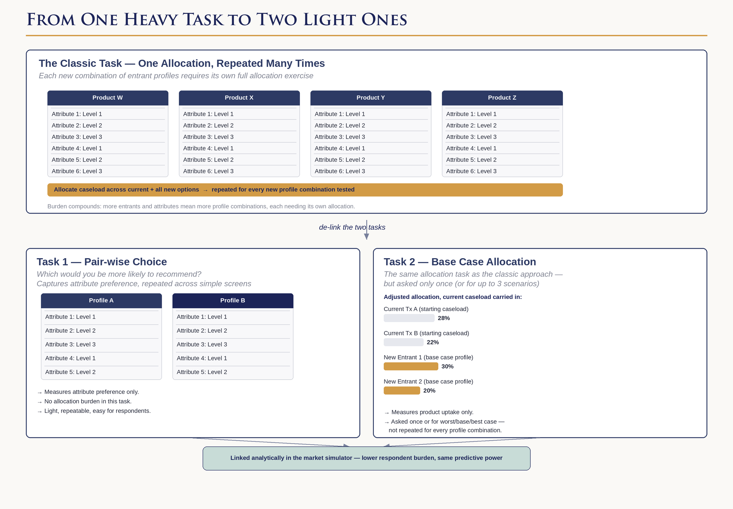
The key insight that leads to practical solutions to these problems of modeling multiple competitive entrants is to recognize that the classic choice model does two things simultaneously:
It measures attribute preference by measuring the trade-offs respondents make
It measures product uptake (i.e., patient share) from the allocation exercise
This works well enough when there are a relatively small number of attributes; however, cognitive burden rises sharply when the task requires respondents to compare multiple new treatments across a large number of attributes. The key is to delink the measurement of attribute preference from product uptake. One way to do this is to measure preferences using a pair-wise discrete choice exercise and measure patient share via a base case scenario containing all newly available treatments. As long as we ensure that the clinical end points for all new treatments in the base case scenario are covered in the range of attributes and levels tested in the pair-wise task, we will be able to link the abstract utilities from the first task with the patient shares from the second task. The end result is similar to what would emerge from a classic choice model but with significantly lower respondent burden and sample requirements. The linkage itself involves using a standard calibration algorithm to generate adjusted ASCs when the attribute preference coefficients are folded into the simulator along with the raw patient shares from the base case scenario.
There are, of course, drawbacks to this approach, mainly that we are relying on one (or sometimes three – a worst-, base- and best-case scenario) allocation exercise to arrive at our estimates of patient share. As with everything, our choice here is to either simplify the design by eliminating certain realities (say, by assuming fixed product profiles for competitive entrants) or to simplify the respondent task using creative approaches and retaining the ability to simulate more realistic future scenarios.
The case of too many attributes
Even the pair-wise approach may require further simplification if the number of attributes exceeds eight[2]. One such simplification is to resort to a partial-profile choice design. In a partial-profile choice model, products are described in terms of a subset of all tested attributes. For example, if there are twelve relevant product attributes, each product profile is described using no more than four to six attributes. Typically, each choice card will contain two partial profiles, and the respondent chooses the one they are most likely to recommend/choose. Respondents are explicitly instructed that the two profiles differ only on the attributes shown; attributes held constant are suppressed from view in the survey programming. Since the partial-profile task measures relative preference from observed trade-offs, respondent assumptions about unshown attributes are analytically irrelevant. The design ensures that each respondent is exposed to all attributes and levels across multiple such scenarios, enabling the model to estimate all main effects reliably. The end result is the same as the full-profile pairwise task as each approach yields utilities that can be linked to patient shares from a limited number of allocation exercises.
Delinking attribute preference measurement from product uptake
Bringing Access into the mix
The most direct way to model the role of access is to incorporate it into the product experimental design using variables such as anticipated restrictions and patient out-of-pocket costs. Depending on the point in the pre-launch process, uncertainties in this arena can be modeled separately with a payor model which is then linked to the HCP model. This is done by modeling the probabilities of various access scenarios amongst payers and using these probabilities as inputs into the HCP model during the simulation stage. This enables us to incorporate access not as discrete levels but as a range of probabilities given different pricing and rebate strategies taken by the launch access team.
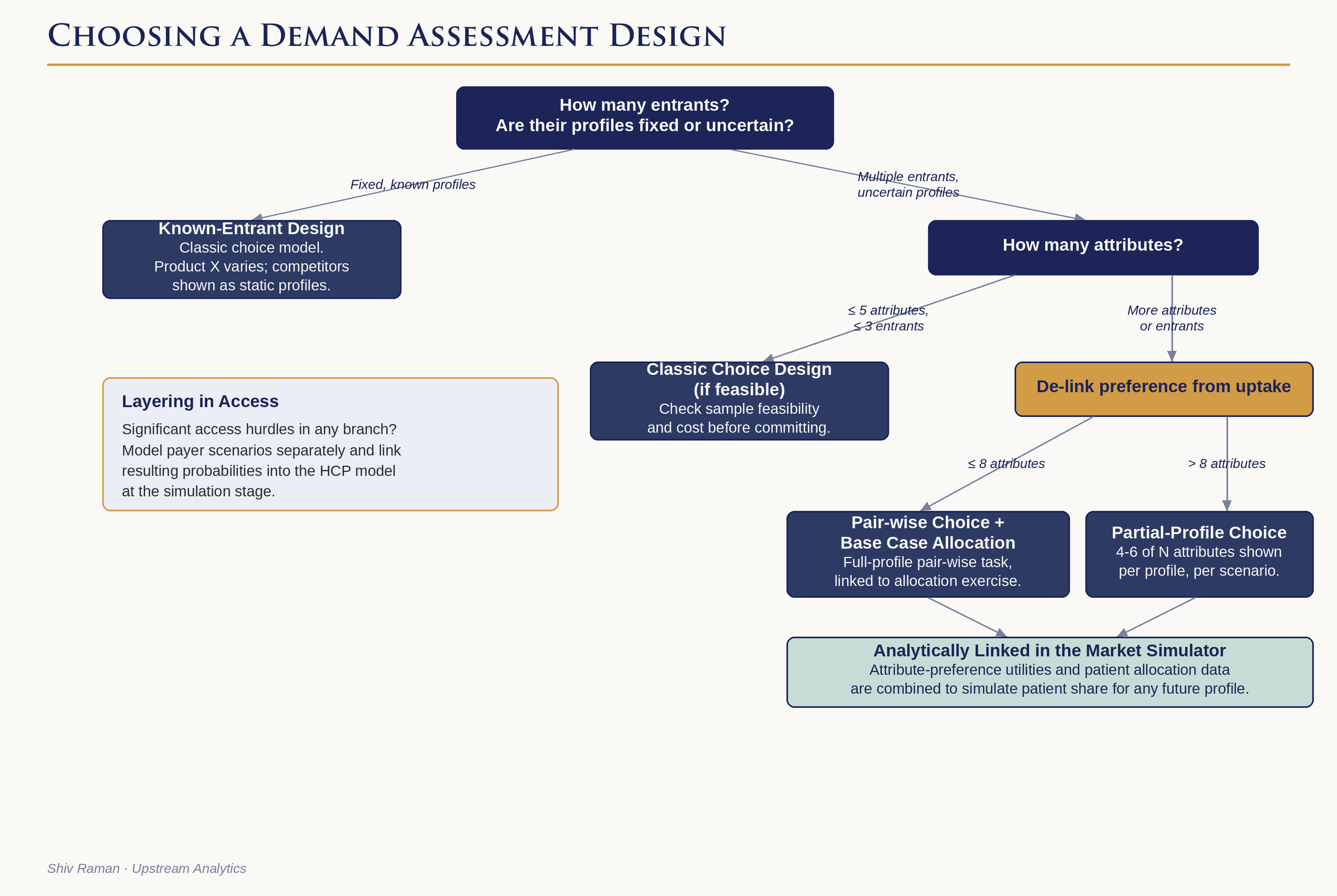
Decision tree to select optimal research design
Putting it all together
To a certain extent it is poetic that trade-off methods require that we ourselves, as researchers have to make several trade-offs, balancing methodological rigor, completeness, efficiency, and cost. Modeling market complexity requires a keen understanding of the priorities of the marketing team, the realities of sampling feasibility, cost and last but not least, the burden on the respondent. There are no simple answers, and a good partner helps the team navigate the trade-offs clearly and arrive at a design that reflects their priorities. Yes, it is the same principle again – almost all the critical decisions happen upstream, well before a single piece of data is collected.
[1] I am ignoring the truly simplest case where we are testing a static profile (or a few discrete variations thereof) as no statistical modeling is involved in estimating patient share.
[2] The exact number may be different depending on the complexity of the attribute levels, but in general, 6-8 are as high as we like to go with a full-profile choice design