
Incorporating a Naïve Bayes Classifier in a Choice Simulator
Introduction
There are problems in market research that look straightforward until you actually try to solve them. A client once asked me to model not just whether physicians would prescribe a new GLP-1 agent, but which dose strength they would choose, and to do so simultaneously, as part of a single choice simulator. While the request appears reasonable on its face, the solution turns out to be not so obvious.
The issue was with the study design: a product with multiple strengths, where all strengths moved in lockstep across levels for certain attributes (for example, if there are three levels of weight loss per strength, all strengths would be at the same level in any given scenario). One might think the natural solution is to treat each strength as a separate alternative in the choice model, and from a mechanistic perspective, this works. The model will estimate strength-specific constants and a common set of attribute coefficients. But those coefficients cannot distinguish between the strengths - they are estimated from the product's overall performance against competitors, not from any variation among the strengths themselves. The strength allocation the model produces therefore does not respond to changes in the product profile being simulated. A simulator whose strength split is the same regardless of what clinical profile is shown is only doing half the job. What was needed was a way to make that allocation dynamic: let the choice model handle product choice and handle the choice of strength as a separate but linked problem.
The solution I landed on was a Naïve Bayes classifier. It is simple, transparent, and grounded entirely in the observed prescribing behavior of the physicians in the study. This article walks through how it works and how it connects to the choice model that sits alongside it.
Designs with nested attributes
Consider the case of a product where different dose strengths have distinctly different efficacy and side effect profiles. In the context of a study in which we are testing the overall product profile on a set of clinical endpoints, the presence of dosage strength-specific outcomes adds significant analytic complications. Let’s take the example of an oral weight loss drug in the GLP-1 class in which a new product is available in three dosage strengths, each with a different impact on HbA1c reduction, weight loss, and GI side effects:
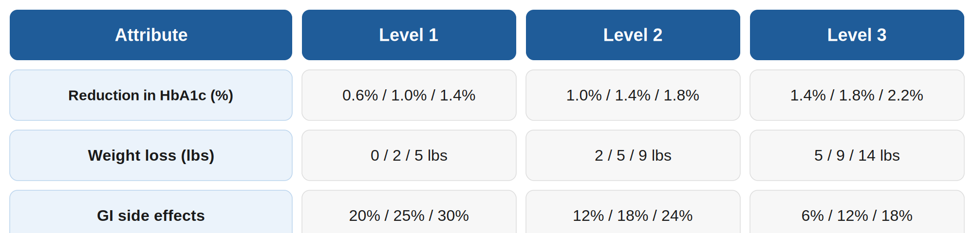
There are additional attributes in the design such as outcomes data, cost, and coverage, but these are not strength dependent. The challenge with this “nested attribute” design is that a physician has to decide not just whether or not to prescribe Product X to a given patient, but also which strength (for simplicity, we assume a discrete choice model, rather than a standard allocation-based model, which is appropriate when HCPs complete the choice exercise in the context of patient records for pre-determined segments). One approach – the classic discrete choice design approach – is to treat each strength as a separate choice alternative and model them simultaneously. This will not work, however, when all attributes are simultaneously at the same level for all strengths. This happens in this case, because a certain level of efficacy (level 1 or 2 or 3) applies to all strengths – i.e., a level three outcome on weight loss means that the three strengths will yield reductions of 5 lbs, 9 lbs, and 14 lbs respectively. This applies to the other dose-dependent attributes as well. And as far as the other attributes are concerned, cost, coverage, etc. it is natural to assume they will not vary by strength.
This poses an analytic problem. Treating each strength as a separate alternative, the model will estimate strength-specific constants alongside attribute coefficients — but since the strengths always appear at identical attribute levels within any given task, those coefficients have no basis for distinguishing between them. The result is a strength allocation anchored to fixed constants that does not shift as the simulated product profile changes. For a simulator whose core purpose is to show how prescribing behavior responds to different clinical configurations, this is a critical limitation.
Enter the Naïve Bayes Classifier
Before we discuss the Bayes Classifier, let’s quickly go over why we are deploying it to solve this problem.
As discussed in the previous section, the choice model can estimate strength-specific constants, and those constants will generate a split of Product X share across the three strengths. But that split is invariant to the product profile: it does not change as the simulator moves between attribute level combinations. Our goal is therefore to replace this fixed allocation with a dynamic one, namely, a mechanism that predicts strength probabilities conditional on the specific profile being simulated. To do this, we separate the probability of choosing Product X from the probability of choosing a particular strength given that Product X was chosen. The choice model handles the former. The Naïve Bayes classifier handles the latter, drawing on the observed prescribing behavior recorded during the choice exercise itself.
A Naïve Bayes classifier is a simple, transparent method for estimating which option is most likely given a set of observed signals. The name deserves a brief explanation:
· Classifier - the method assigns each option (in our case, each dose strength) a probability, effectively ranking them by likelihood. It classifies the most probable outcome given the evidence at hand.
· Bayes - refers to Bayes' theorem, the mathematical rule encoded in the formula described below. It gives us a formal way to update a prior belief in light of new evidence.
· Naïve - the simplifying assumption that the pieces of evidence (here, the three clinical attributes) are treated as independent of one another. In a conjoint study, this is not an assumption at all - it is guaranteed by the experimental design, which varies the attributes independently across choice tasks. The "naïve" label is inherited from broader applications of the method where independence must be assumed; here it holds by construction.
A simple real‑world example helps clarify how priors and likelihoods work together. Imagine walking across a university campus and meeting a student who seems introverted. Suppose that among students who are introverted, the probability of being a Math major is relatively high, perhaps far higher than for most other majors. That is the likelihood: how consistent the observed evidence (introversion) is with each possible major. But Math majors make up only a small fraction of the student body overall. That is the prior: the baseline probability before any evidence is considered. Bayes’ rule combines these two facts. Even though introverted students are disproportionately likely to be Math majors, the updated probability that this particular student is a Math major is still moderated by the fact that Math majors are rare. The posterior reflects both forces: strong evidence pointing toward Math, but a low base rate pulling the probability back. This is exactly the logic the classifier applies when it updates strength probabilities in light of the profile being simulated.
The same three quantities appear in the classifier, stated formally as Bayes' rule:

In plain terms:
P(strength | profile) - the answer we want: given the product profile being simulated, how probable is each strength?
P(strength) - the prior: how often is each strength chosen overall in the data?
P(profile | strength) - the likelihood: how well does the observed profile fit each strength, based on actual strength selections recorded in the exercise?
We multiply the prior by the likelihood for each strength, then rescale the three results so they sum to one. That rescaling step is the only arithmetic beyond simple multiplication, and it gives us a systematic way to estimate the probability of each dose strength, one that responds dynamically to the product profile being simulated. The mechanics of this process, and how the probabilities are computed, are shown in the next section.
Worked example of the Naïve Bayes Simulator
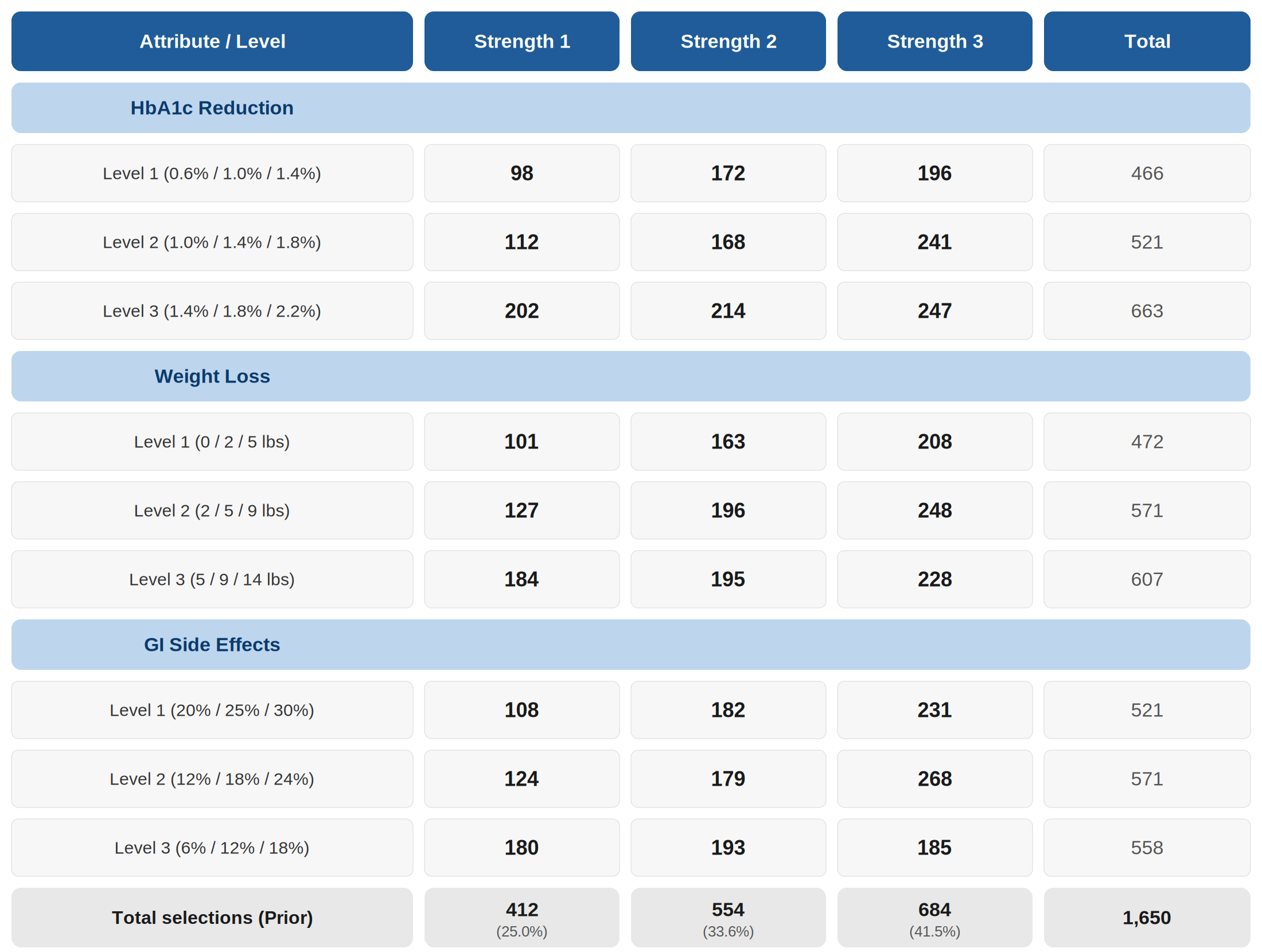
To make the mechanics concrete, we work through a specific simulation scenario using data from the choice exercise. The frequency table below shows the core input to the classifier: for each of the three dose-dependent attributes and each of their three design levels, it records how many times each dose strength was selected by physicians who chose Product X in that task. These counts come directly from observed prescribing behavior in the exercise - not from assumptions or modeling. The prior probability for each strength (bottom row) is simply its overall share of all strength selections across the entire dataset. (Note: attribute levels and frequency counts have been modified from the original study to preserve confidentiality. The analytical structure and methodology are unchanged.)
How the classifier works: a schematic overview
The schematic below shows the complete calculation for a single simulation scenario - HbA1c reduction at Level 1, weight loss at Level 2, and GI side effects at Level 2 - tracing each step from prior to posterior in one view.
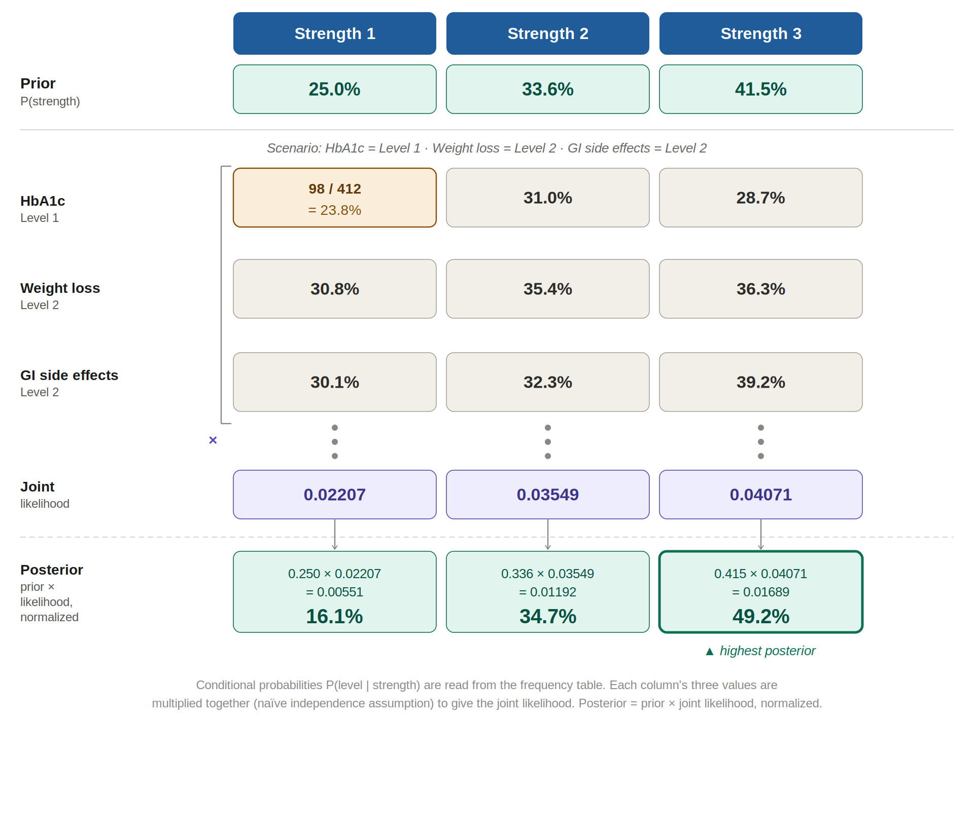
Naïve Bayes classifier schematic. Conditional probabilities are read from the frequency table above. Each column’s three values are multiplied together (the naïve independence step) to yield the joint likelihood. The posterior is prior × joint likelihood, normalized to sum to one.
Reading the schematic
The top row shows the prior probability for each strength - its unconditional share of all 1,650 strength selections in the data (25.0%, 33.6%, and 41.5%). This is the starting point before any profile information is considered.
The three rows of the grid show the conditional probabilities: given the active level of each attribute, how often was each strength selected? The top-left cell makes the arithmetic explicit — 98 physicians chose Strength 1 when HbA1c was at Level 1, out of the 412 total times Strength 1 was selected across the entire exercise, giving a conditional probability of 23.8% - establishing the pattern that all other cells follow. Each percentage is the cell count divided by that strength's total selections - the figures shown in the bottom row of the frequency table.
The vertical ellipsis signals that the three conditional probabilities in each column are multiplied together. This is the naïve step: treating the three attributes as independent signals and combining their evidence by simple multiplication. The result is the joint likelihood for each strength, i.e., how probable the observed combination of attribute levels would be if that strength were the one being prescribed.
The posterior row shows the final output. For each strength, the prior is multiplied by the joint likelihood, and the three resulting values are normalized to sum to one. Under this scenario, Strength 3 emerges as the most probable prescription (49.2%), followed by Strength 2 (34.7%) and Strength 1 (16.1%). The heavier border on Strength 3 marks it as the highest posterior. As the simulator presents different scenarios, all three posteriors shift accordingly.
What the classifier is and is not
The posteriors from the Naïve Bayes classifier are probabilities over strength conditional on Product X being chosen - they are not overall prescription shares. The overall share for each strength is the product of two quantities: the probability that the physician chose Product X at all (from the discrete choice model) and the probability that, having done so, they selected that particular strength (from the classifier). The two models are complementary, and neither is sufficient on its own.
While this example illustrates the total market view, the classifier can be run separately within any physician or patient segment for which sufficient strength selection data is available. A practice pattern that differs meaningfully across patient types, for instance, patients managed primarily on oral agents versus those with prior injectable experience, would yield different posterior distributions, capturing the clinical judgment that physicians apply when selecting a starting dose in the real world.
A principled solution to a practical problem
The Naïve Bayes classifier is not a universal solution to the nested attribute problem. It works when physicians make a two-stage decision (product first, then strength) and when the choice exercise captures both stages explicitly. But in that setting, which arises more often than one might expect in pharmaceutical market research, it fills a genuine gap. It is simple enough to explain to a client, transparent enough to audit, and grounded in observed behavior rather than modeling assumptions. For a simulator that is supposed to show how the world changes as the product profile changes, that combination of properties is exactly what is needed.